

- Introduction
- Analysis in R Studio
Introduction
Customer Churn Prediction in the Telecom Industry by Kaggle
About Dataset
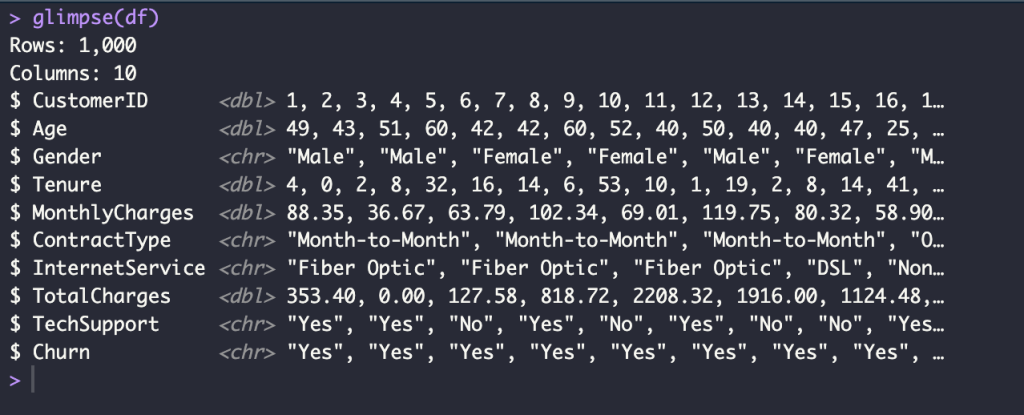
This dataset provides a comprehensive view of customer behavior and churn in the telecom industry. It includes detailed information on customer demographics, service usage, and various indicators that are critical for analyzing customer retention and churn.
- CustomerID : Unique identifier for each customer.
- Age : Age of the customer, reflecting their demographic profile.
- Gender : Gender of the customer (Male or Female).
- Tenure : Duration (in months) the customer has been with the service provider.
- MonthlyCharges : The monthly fee charged to the customer.
- ContractType : Type of contract the customer is on (Month-to-Month, One-Year, Two-Year).
- InternetService: Type of internet service subscribed to (DSL, Fiber Optic, None).
- TechSupport : Whether the customer has tech support (Yes or No).
- TotalCharges : Total amount charged to the customer (calculated as MonthlyCharges * Tenure).
- Churn : Target variable indicating whether the customer has churned (Yes or No).
Analysis in R Studio
Install and Load Package
# Install package
install.packages("tidyverse")
install.packages("caret")
install.packages("gridExtra")

# Load package

library("tidyverse")
library("caret")
library("gridExtra")
library("glue")
Load Data
df <- read_csv("customer_churn_data.csv")
Data Preprocessing
Check data
glimpse(df)
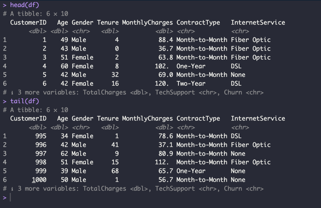
head(df)
tail(df)
names(df)
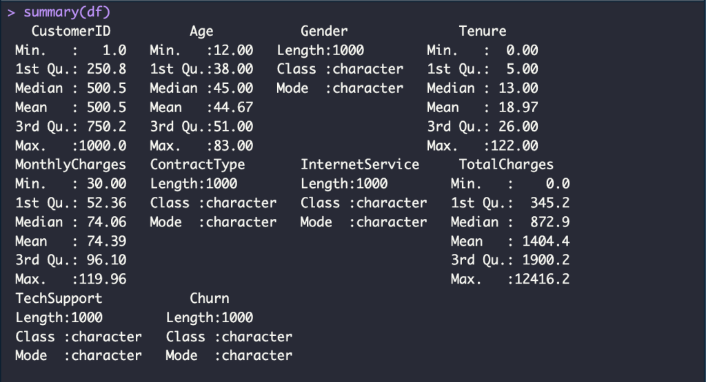
summary(df)
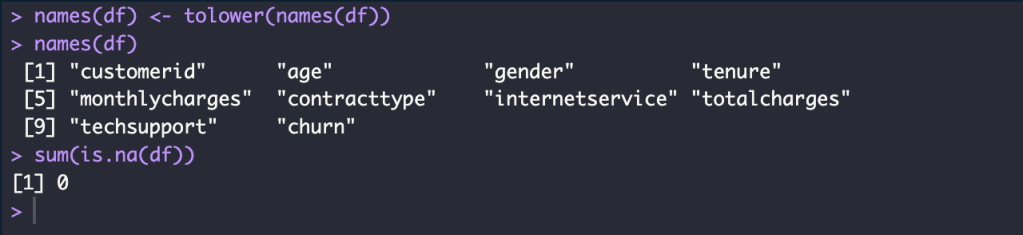
Change column names to lowercase and Check missing value
names(df) <- tolower(names(df))
names(df)

sum(is.na(df))
Create a new data frame without the customerid and techsupport column and Removes all rows containing “None” values
df%>%
  select(internetservice) %>%
  group_by(internetservice) %>%
  count()

df <- df %>%
  select(-1, -9) %>%
  filter(internetservice != "None")

df%>%
  select(internetservice) %>%
  group_by(internetservice) %>%
  count()


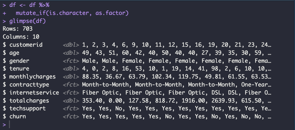
Convert character data type to factor data type
df <- df %>%
  mutate_if(is.character, as.factor)
glimpse(df)
Exploration Data Analysis
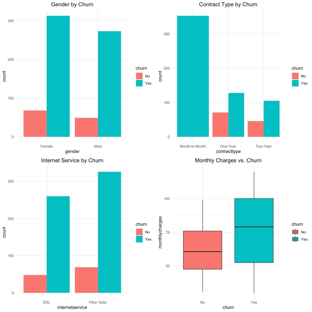
Create the individual plots by ggplot
p1 <- ggplot(df, aes(gender, fill = churn)) +
  geom_bar(position = position_dodge()) +
  theme_minimal() +
  ggtitle("Gender by Churn") +
  theme(plot.title = element_text(hjust = 0.5))

p2 <- ggplot(df, aes(contracttype, fill = churn)) +
  geom_bar(position = position_dodge()) +
  theme_minimal() +
  ggtitle("Contract Type by Churn") +
  theme(plot.title = element_text(hjust = 0.5))

p3 <- ggplot(df, aes(internetservice, fill = churn)) +
  geom_bar(position = position_dodge()) +
  theme_minimal() +
  ggtitle("Internet Service by Churn") +
  theme(plot.title = element_text(hjust = 0.5))

p4 <- ggplot(df, aes(churn, monthlycharges, fill = churn)) +
  geom_boxplot() +
  theme_minimal() +
  ggtitle("Monthly Charges vs. Churn") +
  theme(plot.title = element_text(hjust = 0.5))
Arrange the plots in a grid
grid.arrange(p1, p2, p3, p4, ncol = 2)
Build Machine Learning Model
Split Data
Train Data 80 % and Test Data 20 %
set.seed(42)
n <- nrow(df)
id <- sample(1:n, size = 0.8*n, replace = FALSE)
train_data <- df[id, ]
test_data <- df[-id, ]
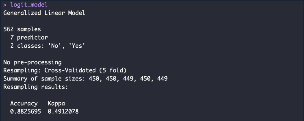
Logistic Regression with K-Fold CV
Train Model
set.seed(42)
ctrl <- trainControl(method = "cv",
                     number = 5)
logit_model <- train(churn ~ .,
                     data = train_data,
                     method = "glm",
                     trControl = ctrl)
accuracy_logit_train <- round(logit_model$results$Accuracy, 4)*100
accuracy_logit_train_p <- glue("{accuracy_logit_train}%")
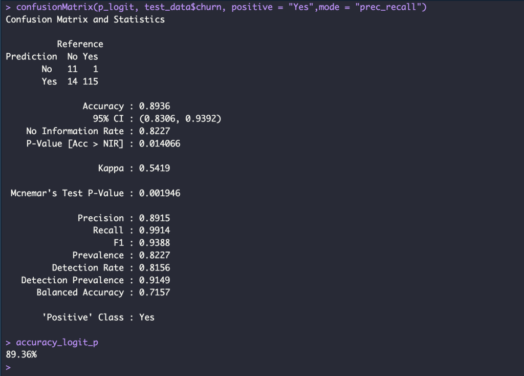
Test Model
p_logit <- predict(logit_model, newdata = test_data)

confusionMatrix(p_logit, test_data$churn, positive = "Yes",mode = "prec_recall")

accuracy_logit <- round(mean( p_logit == test_data$churn), 4)*100
accuracy_logit_p <- glue("{accuracy_logit}%")
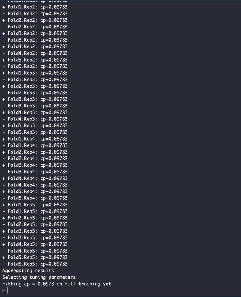
Decision Tree with Repeated K-Fold CV
Train Model
set.seed(42)
ctrl <- trainControl(method = "repeatedcv",
repeats = 5,
number = 5,
verboseIter = TRUE)
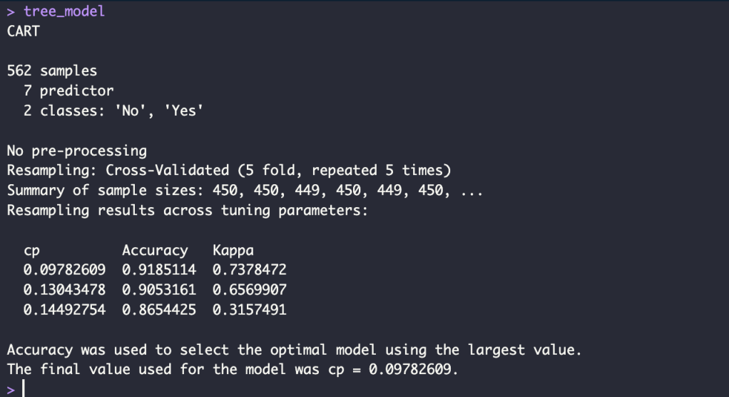
tree_model <- train(churn ~ .,
data = train_data,
method = "rpart",
trControl = ctrl)
accuracy_tree_train <- round(max(tree_model$results$Accuracy), 4)*100
accuracy_tree_train_p <- glue("{accuracy_tree_train}%")
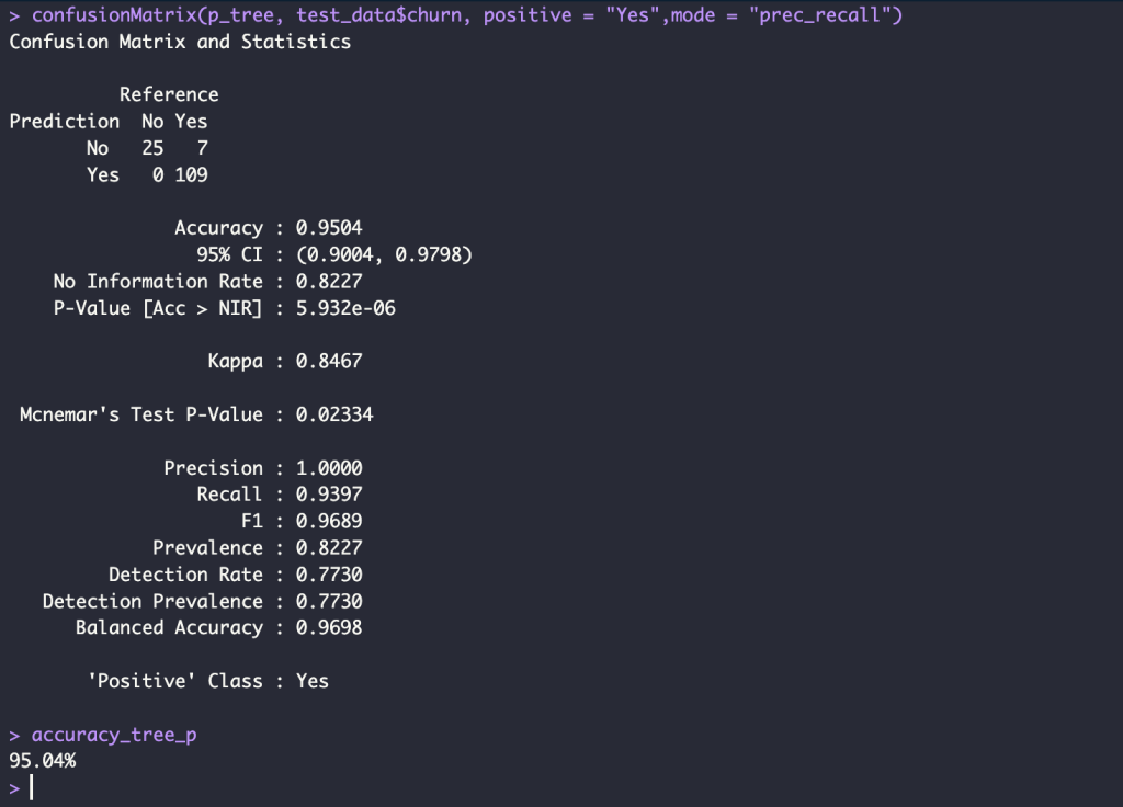
Test Model
p_tree <- predict(tree_model, newdata = test_data)

confusionMatrix(p_tree, test_data$churn, positive = "Yes",mode = "prec_recall")

accuracy_tree <- round(mean( p_tree == test_data$churn),4)*100

accuracy_tree_p <- glue("{accuracy_tree}%")
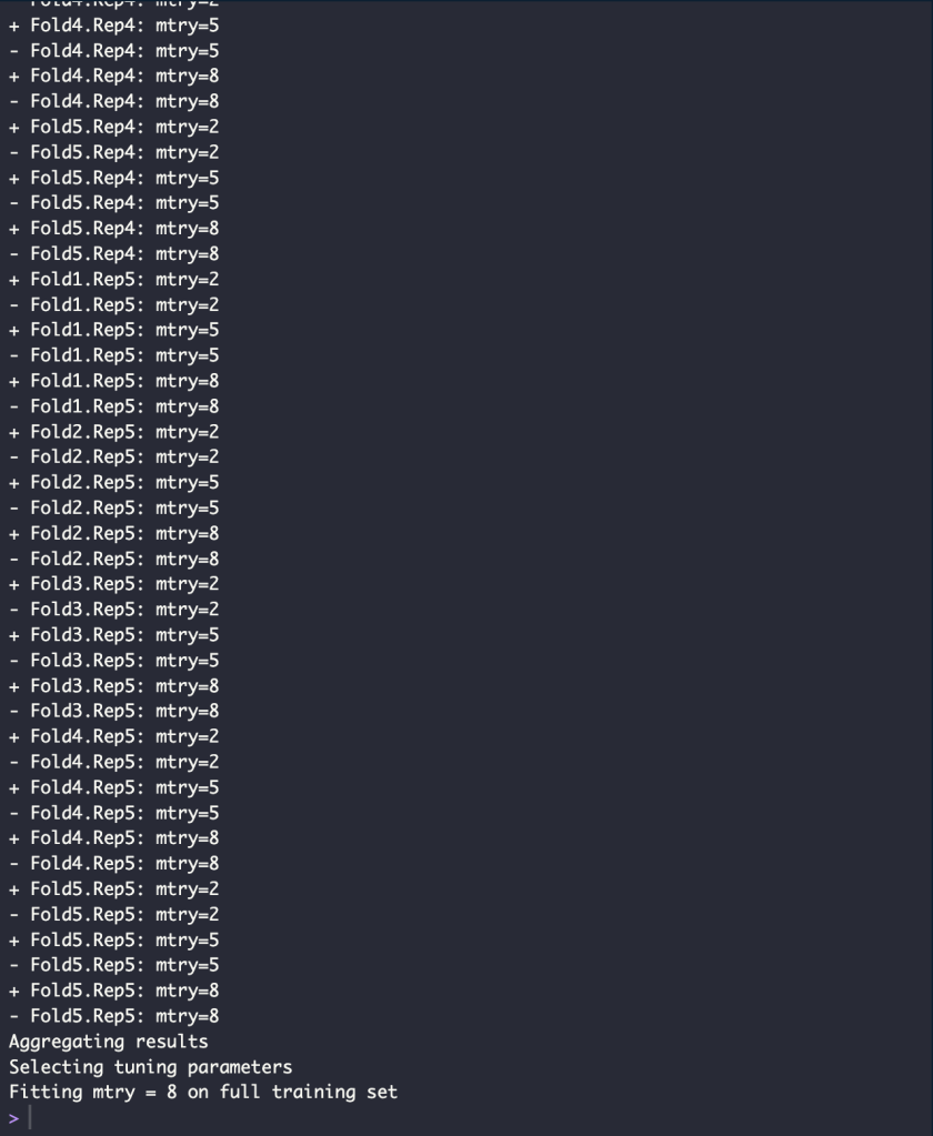
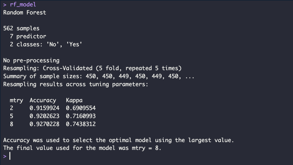
Random Forest with Repeated K-Fold CV
Train Model
set.seed(42)
ctrl <- trainControl(method = "repeatedcv",
                     repeats = 5,
                     number = 5,
                     verboseIter = TRUE)
rf_model <- train(churn ~ .,
                    data = train_data,
                    method = "rf",
                    trControl = ctrl)
accuracy_rf_train <- round(max(rf_model$results$Accuracy), 4)*100
accuracy_rf_train_p <- glue("{accuracy_rf_train}%")
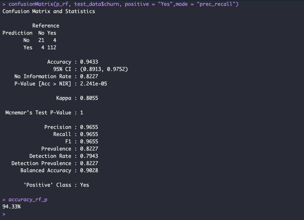
Test Model
p_rf <- predict(rf_model, newdata = test_data)

confusionMatrix(p_rf, test_data$churn, positive = "Yes",mode = "prec_recall")

accuracy_rf <- round(mean( p_rf == test_data$churn), 4) * 100
accuracy_rf_p <- glue("{accuracy_rf}%")
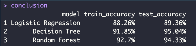
Conclusion Accuracy
conclusion <- data.frame(
  model = c("Logistic Regression", "Decision Tree", "Random Forest"),
  train_accuracy = c(accuracy_logit_train_p, accuracy_tree_train_p, accuracy_rf_train_p),
  test_accuracy = c(accuracy_logit_p, accuracy_tree_p, accuracy_rf_p)
)

Leave a comment