

- Introduction
- Analysis in R Studio
Introduction
Student Performance Factors by Kaggle
About Dataset
This dataset provides a comprehensive overview of various factors affecting student performance in exams. It includes information on study habits, attendance, parental involvement, and other aspects influencing academic success.
- Hours_Studied : Number of hours spent studying per week.
- Sleep_Hours : Average number of hours of sleep per night.
- Previous_Scores : Scores from previous exams.
- Family_Income : Family income level (Low, Medium, High).
- Parental_Education_Level : Highest education level of parents (High School, College, Postgraduate).
- Distance_from_Home : Distance from home to school (Near, Moderate, Far).
- Gender: Gender of the student (Male, Female).
- Exam_Score : Final exam score.
- Attendance : Percentage of classes attended.
- Tutoring_Sessions : Number of tutoring sessions attended per month.
Analysis in R Studio
Install and Load Package
# Install package
install.packages("tidyverse")
install.packages("caret")
install.packages("gridExtra")
install.packages("metan")

# Load package

library("tidyverse")
library("caret")
library("gridExtra")
library("metan")
Load Data
df <- read_csv("StudentPerformanceFactors.csv")
Data Preprocessing
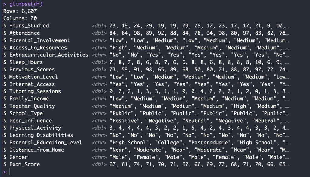
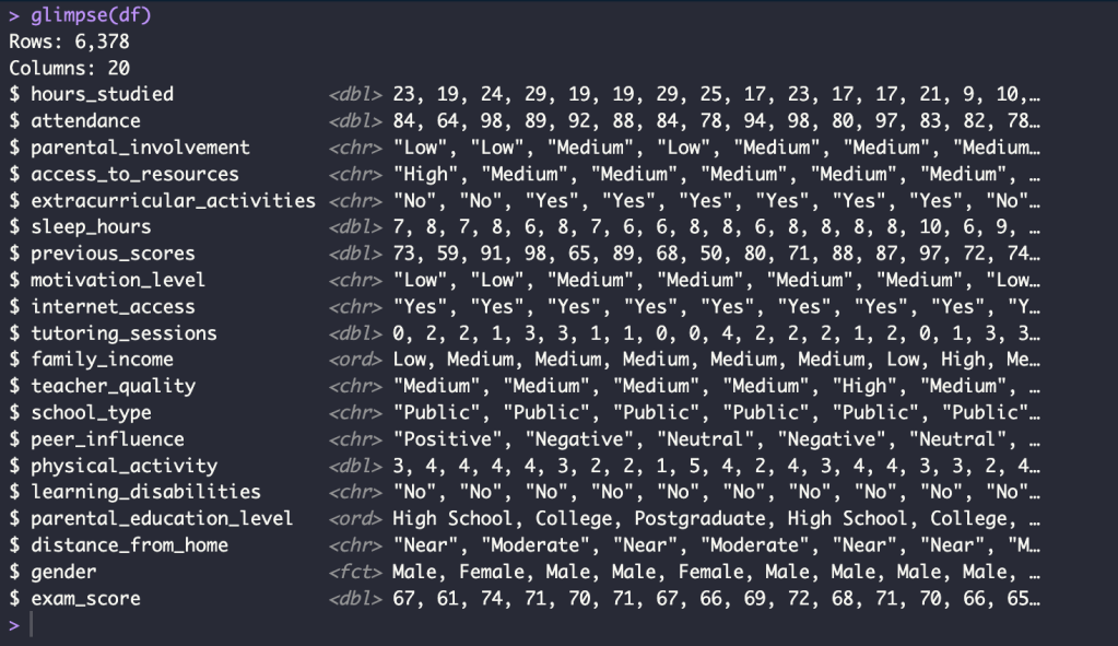
glimpse(df)
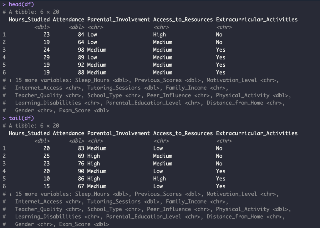
head(df)
tail(df)
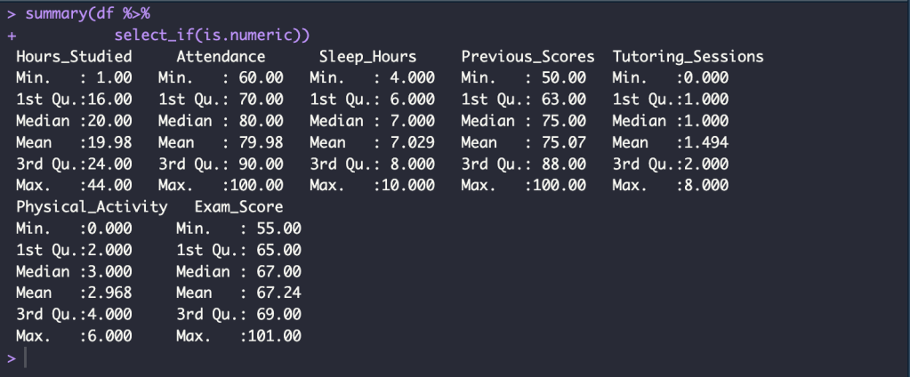
summary(df %>%
select_if(is.numeric))
Change column names to lowercase and Check missing value
names(df) <- tolower(names(df))
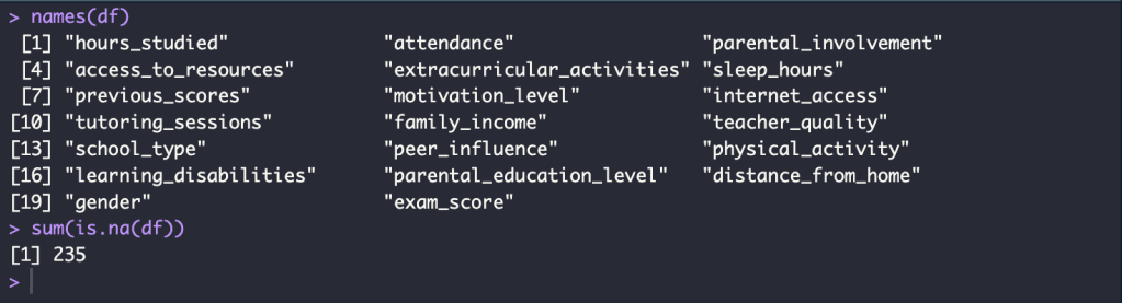
names(df)
sum(is.na(df))
Delete Missing Value
df <- na.omit(df)
sum(is.na(df))
Select only columns that are NOT character data type
df_numeric <- df %>%
  select_if(negate(is.character))
Convert character data type to factor data type
df$family_income <- factor(df$family_income,
                       levels = c("Low","Medium","High"),
                       labels = c("Low","Medium","High"),
                       ordered = T)
df$parental_education_level <- factor(df$parental_education_level,
                           levels = c("High School","College","Postgraduate"),
                           labels = c("High School","College","Postgraduate"),
                           ordered = T)
df$gender <- as.factor(df$gender)
Exploration Data Analysis
Create the individual plots by ggplot
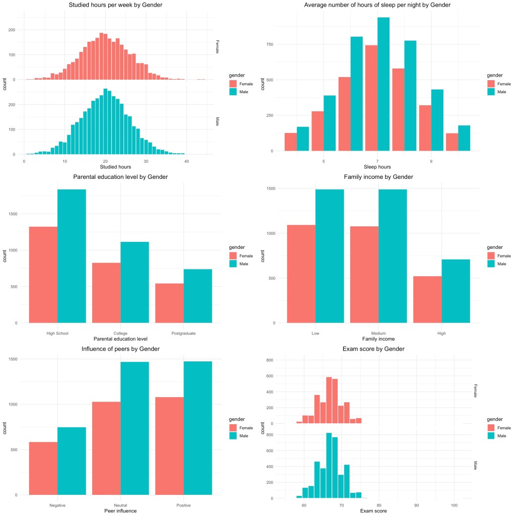
p1 <- ggplot(df, aes(hours_studied, fill = gender)) +
  geom_bar() +
  theme_minimal() +
  facet_grid(gender ~ .) +
  labs(title = "Studied hours per week by Gender",
       x = "Studied hours") +
  theme(plot.title = element_text(hjust = 0.5))


p2 <- ggplot(df, aes(sleep_hours, fill = gender)) +
  geom_bar(position = position_dodge()) +
  theme_minimal() +
  labs(title = "Average number of hours of sleep per night by Gender",
     x = "Sleep hours") +
  theme(plot.title = element_text(hjust = 0.5))


p3 <- ggplot(df, aes(parental_education_level  , fill = gender)) +
  geom_bar(position = position_dodge()) +
  theme_minimal() +
  labs(title = "Parental education level by Gender",
       x = "Parental education level") +
  theme(plot.title = element_text(hjust = 0.5))


p4 <- ggplot(df, aes(family_income  , fill = gender)) +
  geom_bar(position = position_dodge()) +
  theme_minimal() +
  labs(title = "Family income by Gender",
       x = "Family income") +
  theme(plot.title = element_text(hjust = 0.5))


p5 <- ggplot(df, aes(peer_influence  , fill = gender)) +
  geom_bar(position = position_dodge()) +
  theme_minimal() +
  labs(title = "Influence of peers by Gender",
       x = "Peer influence") +
  theme(plot.title = element_text(hjust = 0.5))


p6 <- ggplot(df, aes(exam_score, fill  = gender)) +
  geom_histogram(color = "white") +
  theme_minimal() +
  facet_grid(gender ~ .) +
  labs(title = "Exam score by Gender",
       x = "Exam score") +
  theme(plot.title = element_text(hjust = 0.5))
Arrange the plots in a grid
grid.arrange(p1, p2, p3, p4, p5, p6, ncol = 2)
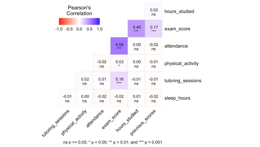
Correlation Matrix
Build Machine Learning Model
Split Data
Train Data 80 % and Test Data 20 %
set.seed(42)
n <- nrow(df)
id <- sample(1:n, size = 0.8*n, replace = FALSE)
train_data <- df[id, ]
test_data <- df[-id, ]
Linear regression with K-Fold CV
Train Model
set.seed(42)
ctrl <- trainControl(method = "cv",
                     number = 5,
                     verboseIter = TRUE)
lm_model <- train(exam_score ~ previous_scores + hours_studied + attendance + tutoring_sessions,
                  data = train_data,
                  method = "lm",
                  trControl = ctrl)

Test Model
p_lm <- predict(lm_model, newdata = test_data)

rmse_lm <- sqrt(mean( (p_lm - test_data$exam_score)**2 ))
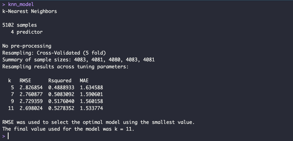
KNN with K-Fold CV
Train Model
set.seed(42)
ctrl <- trainControl(method = "cv",
number = 5,
verboseIter = TRUE)
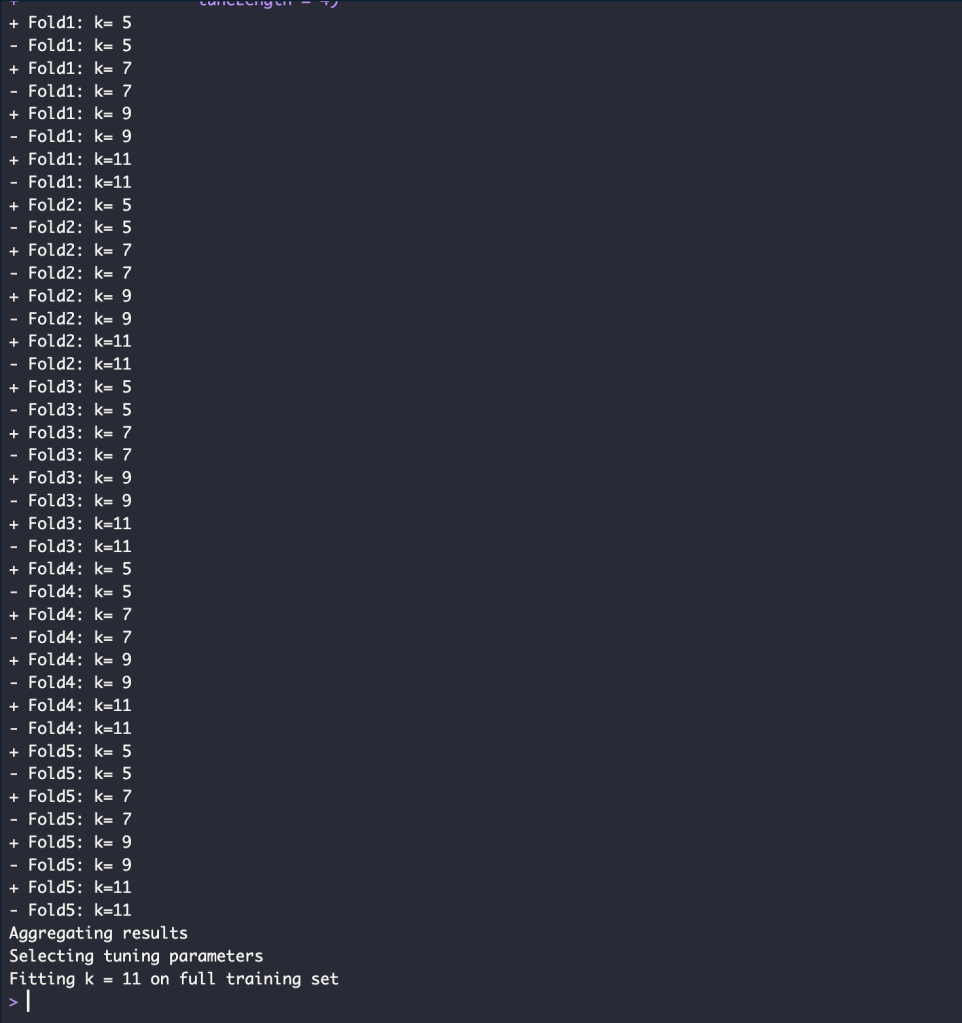
knn_model <- train(exam_score ~ previous_scores + hours_studied + attendance + tutoring_sessions,
data = train_data,
method = "knn",
trControl = ctrl,
tuneLength = 4)
Test Model
p_knn <- predict(knn_model, newdata = test_data)

rmse_knn <- sqrt(mean( (p_knn - test_data$exam_score)**2 ))
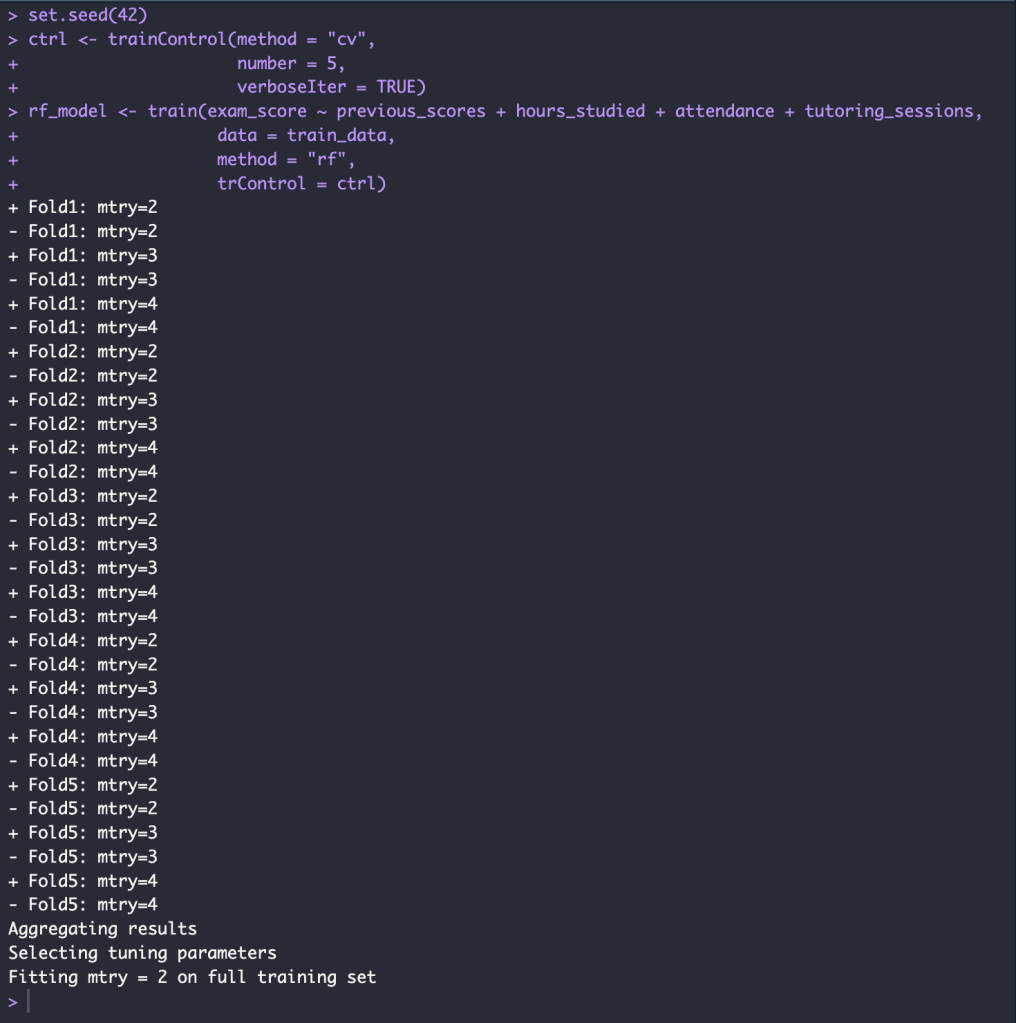
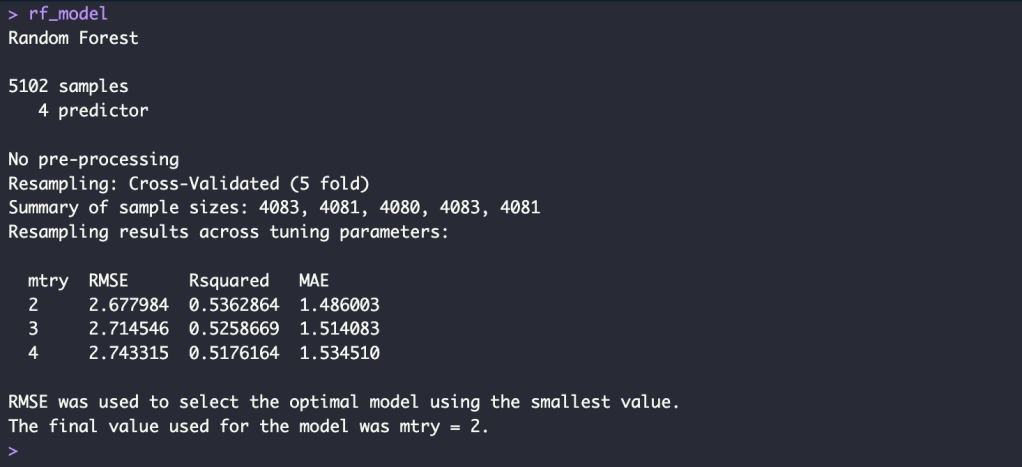
Random Forest with K-Fold CV
Train Model
set.seed(42)
ctrl <- trainControl(method = "cv",
                     number = 5,
                     verboseIter = TRUE)
rf_model <- train(exam_score ~ previous_scores + hours_studied + attendance + tutoring_sessions,
                   data = train_data,
                   method = "rf",
                   trControl = ctrl)
Test Model
p_rf <- predict(rf_model, newdata = test_data)

rmse_rf <- sqrt(mean( (p_rf - test_data$exam_score)**2 ))
Conclusion RMSE
conclusion <- data.frame(
  model = c("Linear regression with K-Fold CV","KNN with K-Fold CV", "Random Forest with K-Fold CV "),
rmse_train = c("2.543691", "2.698024", "2.677984"),
rmse_test = c("2.218041", "2.397026", "2.383069")
)

print(conclusion)


Leave a comment